Given the Probability Density Function for a Continuous Random Variable X Àµ†ž Àµ Ý” ž Àµ

Given a random experiment, with a sample space, \(S\), we can define the possible values of \(S\) as a random variable. In other words, a random variable can be defined as a numerical quantity whose value is determined by chance. Random variables can be either discrete or continuous.

Discrete Random Variables

A discrete random variable is a variable whose range of possible values is from a specified list. In other words, a discrete random variable takes distinct countable numbers of positive values in the sample space, and it is not possible to get values between the numbers.

For a discrete variable \(X\), we define the probability mass function (PMF) as a function that describes the relationship between the random variable, \(X\), and the probability of each value of \(X\) occurring. The PMF of \(X\) is mathematically defined as:

$$f\left(a\right)=P(X=a)$$

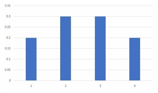
The probability mass function is usually presented graphically by plotting \(f(x_i)\) on the y-axis against \(x_i\) on the x-axis. For example, the probability massdensity function shown in the graph below can be written as:

$$ f\left( x \right) =\begin{cases} 0.2, & x=1,4 \\ 0.3, & x=2,3 \end{cases} $$

The probability mass function of a discrete random variable has the following properties:

1. \(f \left(x \right) > 0,\quad x € S;\) meaning all individual probabilities must be greater than zero.
2. \({ \Sigma }_{ x\in S }f\left( x \right)=1; \) meaning the sum of all individual probabilities must equal one.
3. \(P\left( X\in A \right) ={ \Sigma }_{ x\in A }f\left( x \right) \),where \(A\subset S; \) meaning the probability of event \(A\) is the sum of the probabilities of the values of \(X\) in \(A\).

Example: Discrete Random Variable

Suppose a customer care desk receives calls at a rate of 3 calls every 4 minutes. Assuming a Poisson process, what is the probability of receiving 4 calls within a 16-minutes period?

Solution

We know that for a Poisson random variable

$$ P(X=k)=\frac {(\lambda^k e^{(-\lambda)})}{k!} $$

In this case,

$$ \lambda=\frac{3}{4}\times16=12 $$

Thus,

$$ P\left(X=4\right)=\frac{{12}^4e^{-12}}{4!} =0.0053 $$

Cumulative Distribution Function for Discrete Random Variables

For a random variable \(X\), the cumulative distribution function of \(X\) can be defined as

$$ F\left( x \right) =P\left( X\le x \right) ,\quad \quad -\infty <x<\infty $$

The cumulative distribution function \(F\) for a discrete random variable can be expressed in terms of \(f(a)\) as:

$$F\left(a\right)=\sum_{\forall\ x\le a}{f(x)}$$

For a discrete random variable \(X\) whose possible values are \(x_1,x_2,x_3,\ldots\) for all \(x_1<x_2<x_3<\ldots\), the cumulative distribution function \(F\) of \(X\) is a step function. As such, \(F\) is constant in the interval \([x_{i-1},\ x_i]\) and take a lip (jump) of \(f(x_i)\) at \(x_i\).

Example: Graph of Cumulative Distribution Function

Consider the following probability distribution:

$$f(x)=\begin{cases}0.2,&x=1,4\\ 0.3, & x=2,3\\\end{cases}$$

Compute the cumulative distribution and plot its graph.

Solution

Consider the following table:

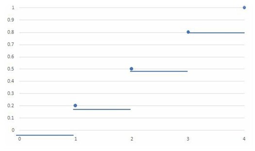
$$ \begin{array}{c|c|c|c} \bf{X_i} & \bf{f(x_i)} & \bf{F(x_i)}  \\ \hline 1 & 0.2 & 0.2  \\ \hline 2 & 0.3 & 0.5  \\ \hline 3 & 0.3 & 0.8  \\ \hline 4 & 0.2 & 1.0  \\ \end{array} $$

The above results can be represented as:

$$ F\left( x \right) =\begin{cases} 0, & x<1 \\ 0.2, & 1\le x<2 \\ 0.5, & 2\le x<3 \\ 0.8, & 3\le x<4 \\ 1, & x\ge 4 \end{cases} $$

The graph of the cumulative distribution function is as shown below:

Continuous Random Variable

A continuous random variable is a random variable that has an infinite number of possible values. For a continuous random variable \(X\), we define a non-negative function \(f(x)\) for all \(x\in(-\infty,\infty)\) with the property that for all real values \(R\),

$$\Pr{\left(X\in R\right)}=\int_{R}{f(x)}\ dx$$

The probability density function (pdf), \(f(x)\), of a continuous random variable is a differential equation with the following properties:

1. \(f\left( x \right)\ge 0\): meaning the function (all probabilities) is always greater than zero.

   \(\int _{ -\infty }^{ \infty }{ f\left( x \right)dx=1 } \): meaning the sum of all the possible values (probabilities) is one.

It is important to note that while the probability mass function of a discrete random variable is a probability value, the probability density function of a continuous random variable is not a probability. Therefore, for continuous random variables, we can get the desired probability value from a given probability density function, using the following function:

$$ P\left( X < a \right) =P\left( X\le a \right) =f\left( a \right) =\int _{ -\infty }^{ a }{ f\left( x \right) dx } $$

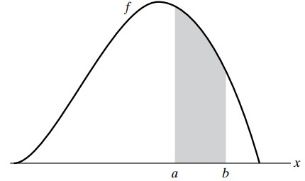
Also note that, for \(R=\left[a,b\right]\)

$$ P\left(a\le X\le b\right)=\int_{a}^{b}{f\left(x\right)\ dx} $$

The graph  of  \(P\left(a\le X\le b\right)\) is as shown below:

Also, it is important to note that the probability of any individual value of a probability density function is zero, as shown in the formula below:

$$P\left(X=a\right)= \int_{a}^{a}{f\left(x\right)} dx=0$$

Example: Calculating Probability from a PDF

Given the following probability density function of a continuous random variable:

$$ f\left( x \right) =\begin{cases} { x }^{ 2 }+c, & 0 < x < 1 \\ 0, & \text{otherwise} \end{cases} $$

1. Calculate C.

   Solution

   Using the fact that:

   $$\begin{align*} \int_{-\infty}^{\infty}{f(x)dx} & =1 \\ \Rightarrow \int _{ 0 }^{ 1 }{ \left( { x }^{ 2 }+C \right) dx} & =1 \\ = { \left[ \frac { { x }^{ 3 } }{ 3 } +Cx \right] }_{ x=0 }^{ x=1 } & =1 \\ = \frac {{1}}{{3}} + C & = 1 \\ \therefore C & = \frac {{2}}{{3}} \end{align*}$$

2. Calculate \(P (X > {\frac {1}{2})}\)

   We know that:

   $$ \begin{align*} P\left(X > a\right) & = \int_{a}^{\infty}f\left(x\right)dx \\ \Rightarrow P\left(X > \frac{1}{2}\right) & =\int_{\frac{1}{2}}^{1}{(x^2+\frac{2}{3})dx} \\ & =\left[\frac{x^3}{3}+\frac{2}{3}x\right]_{x=\frac{1}{2}}^{x=1} \\ & =\left[\frac{1}{3}+\frac{2}{3}\right]-\left[\frac{1}{24}+\frac{1}{3}\right] \\ & =0.625 \end{align*}$$

The Cumulative Distribution Function – Continuous Case

Just like for discrete random variables, the cumulative distribution function of \(X\) can be defined as

$$ F(x) = P(X \le x) ,-\infty < x < \infty $$

However, while summation is applied for discrete calculations, integration is applied for continuous random variables. i.e.,

$$ F (x) =\int_{-\infty}^{x}f\left(x\right)dx $$

Example: Cumulative Distribution Function-Continuous Case

Given the following PDF,

$$ f(x)= \begin{cases} x^2+c, & 0 < x < 1 \\ 0, & \text{otherwise} \end{cases} $$

Find the cumulative distribution function, \(F(x)\).

Solution

From the previous example, we had calculated that \(c=\frac{2}{3}\)

$$ \Rightarrow f(x)= \begin{cases} x^2+\frac{2}{3}, & 0 < x < 1 \\ 0, & \text{otherwise} \end{cases} $$

Therefore,

$$ F\left(x\right) = \begin{cases} \int_{-\infty}^x 0 \ dt=0, & \text{for } x < 0 \\ \int_{-\infty}^0 0 \ dt+ \int_0^x \left(t^2+\frac{2}{3} \right)dt=\frac{x^3}{3}+\frac{2}{3}x, & \text{for } 0 < x < 1 \\ \int_{-\infty}^{0} 0 \ dt+ \int_0^1 \left(t^2+\frac{2}{3}\right)dt+ \int_1^x 0 \ dt=1, & \text{for } x \ge 1 \end{cases} $$

Conditional Probability

Conditional probabilities of random variables can be calculated in a similar way to empirical conditional probabilities, as shown in the formula below:

$$ P\left( A|B \right) =\frac { P\left( A\cap B \right) }{ P\left( B \right) } $$

For example, let event \(A\) be \(X > 2\) and event \(B\) be \(X < 4\), then

$$ P\left( A|B \right) =\frac { P\left( 2<X<4 \right) }{ P\left( X<4 \right) } $$

Example: Calculating Conditional Probability

Given the following probability density function of a continuous random variable:

$$ f\left( x \right) =\begin{cases} { x }^{ 2 }+ \frac {2}{3}, & 0 < x < 1 \\ 0, & \text{otherwise} \end{cases} $$

Calculate \( {P} \left({ {X} }<\cfrac{3}{4}∣{ {X} }>\cfrac{1}{2}\right) \)

Solution

Using the fact that:

$$ \begin{align*} P\left(A\mid B\right) & =\frac{P\left(A\cap B\right)}{P\left(B\right)} \\ \Rightarrow P \left(X < \frac{3}{4}\mid X > \frac{1}{2} \right) & = \frac{P \left(X < \frac{3}{4}\cap X >\frac{1}{2}\right)}{P \left(X > \frac{1}{2} \right)} \\ & =\frac{P\left(\frac{1}{2} < X < \frac{3}{4}\right)}{P(X > \frac{1}{2})} \end{align*} $$

Now,

$$ \begin{align*} P\left(\frac{1}{2} < X < \frac{3}{4}\right)& =\int_{\frac{1}{2}}^{\frac{3}{4}}\left(x^2+\frac{2}{3}\right)dx \\ & =\left[\frac{x^3}{3}+\frac{2}{3}x\right]_{x=\frac{1}{2}}^{x=\frac{3}{4}}=0.265625 \\ P\left(X > \frac{1}{2}\right)& =\int_{\frac{1}{2}}^{1}\left(x^2+\frac{2}{3}\right)dx=\left[\frac{x^3}{3}+\frac{2}{3}x\right]_{x=\frac{1}{2}}^{x=1}=\frac{5}{8} \\ \Rightarrow P \left(X < \frac{3}{4}\mid X > \frac{1}{2}\right) & =\frac{0.265625}{\frac{5}{8}}=0.425 \end{align*} $$

Learning Outcome

Topic 2.a – b: Univariate Random Variables – Explain and apply the concepts of random variables, probability, and probability density functions, cumulative distribution functions & Calculate conditional probabilities.

manzojohispent1945.blogspot.com

Source: https://analystprep.com/study-notes/actuarial-exams/soa/p-probability/univariate-random-variables/explain-and-apply-the-concepts-of-random-variables/

Share this post